Live Plot Sensor Data on TFT Display ILI9486 using ESP32

We all have some IoT projects in mind where we want to have a great visual communication with the users. TFT display are the best means if you want to convey the information visually in your absence. There are libraries for designing stunning GUI for TFT display, like
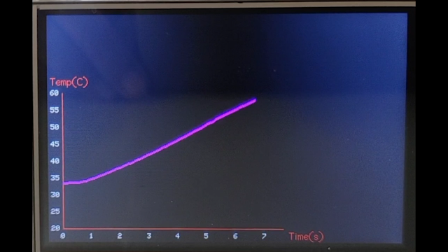
GUISclice. But my project involved display of information in a graphical format. Herein I wanted to display the sensor data during a material testing operation. The end result can be seen in the video. I had the empty space on top and right for some other stuff.
Hardware and Libraries
Before we begin, let's have the look at the hardware and library stuff. Our display is an Arduino board comparable, 480 x 320, 3.5 inch, Touch TFT with serial communication protocol. For our controller, we are using the IoT enable ESP32.
Getting the Touch working with ESP32 in serial mode is tricky, and I will write a post on this latter. Right now, let's focus on the display part
We are using an excellent library TFT_eSPI from Bodmer. Further, I have used the Graph example as my starting point and made necessary changes.
Let's begin! - The complete code is accessible Here
The Plot Function
We will create a plot function which can be called each time a new sensor data is available and needs to be plotted on the display.
We are using a Circular Buffer library for Arduino for easy array management. This array holds the data to be plotted.
- First, we create a plot or graph area, the axis values and labels. Here, we use the final axis limits in case of static axis limits - (Temperature 20 - 60). Else, we use a minimum axis range in case of dynamic axis limit (Time 0 - 1), as the data comes in the time axis will expand and change dynamically.
Graph(tft, xplot, yplot, 1, 20, 300, 300, 192, 0, 1, 1, 20, 60, 5, "", "Time(s)", "Temp(C)", display1, YELLOW, WHITE);
We will create a plot function which can be called each time a new sensor data is available and needs to be plotted on the display.
-
Now, to update the graph, we will find the min and max values from the data array. This is needed to generate the lower and upper limit of an axis (for dynamic axis)
-
We then create black rectangle fills to wipe the old plot, before a new one is created. This is to hide old plot marking from plot area. You may need to perform some calculation or do trial and error to optimize this.
tft.fillRect(startX, startY, width, height, FillColor)
-
Then we iterate through each point in the data array and plot the same. In the plot function, we use the min and max values to determine the dynamic axis range.
-
In case you want to hide the axis text, pass a BLACK text color, and it won't be visible on the display
void plotGraphP()
{
  // Iteratig through the buffer to find the min and max values to be used in creating the axis limits dumanically
  for (int z = 0; z < plotTemp.size(); z++)
  {
    minX = min(minX, plotTime[z]);
    maxX = max(maxX, plotTime[z]);
    // minY = min(minY, plotTemp[z]); // my y axis is static so dont need to find the min max to generate the axis limit
    // maxY = max(maxY, plotTemp[z]); // my y axis is static so dont need to find the min max to generate the axis limit
  }

  update1 = true;
  tft.fillRect(21, 100, 310, 199, BLACK); // need to wipe graph before each update else old traces will show, calculate or trial and error your coordinates
  tft.fillRect(25, 301, 300, 20, BLACK);  // x axis wiping is required as my x axis is dynamic
  // tft.fillRect(0, 100, 17, 195, BLUE ); // y axis is stable for me so no wiping: Hint - use visible color to wipe to see the area that is wiped (for testing)

  for (int u = 0; u < plotTemp.size(); u++)
  {
    yplot = plotTemp[u];
    xplot = plotTime[u];
    Trace(tft, xplot, yplot, 1, 20, 300, 300, 192, minX, (maxX + 1), 1, 20, 60, 5, "", "", "", update1, PINK, WHITE);
    // Textcolor BLACK can be passed to hide it from viewing
    // Do not update axis lables if not necessary
  }
}
As mentioned earlier, the plot function can be called on sensor data receive. Here we are using an array with data to simulate sensor readings. So the plotting can be triggered as
double initplotTemp[81] = {33.42, 33.42, 33.46, 33.55, 33.55, 33.57, 33.57, 33.73, 33.84, 33.96, 34.16, 34.4, 34.6, 34.88, 35.17, 35.45, 35.7, 35.89, 36.28, 36.59, 36.84, 37.2, 37.51, 37.74, 38.1, 38.35, 38.7, 39, 39.34, 39.57, 39.95, 40.23, 40.57, 40.91, 41.23, 41.5, 41.91, 42.21, 42.53, 42.96, 43.24, 43.59, 44.03, 44.28, 44.65, 45.03, 45.35, 45.65, 46.13, 46.48, 46.86, 47.23, 47.67, 48.01, 48.36, 48.76, 49.16, 49.55, 49.91, 50.31, 50.74, 51.07, 51.43, 51.83, 52.3, 52.63, 52.98, 53.34, 53.69, 53.98, 54.41, 54.77, 55.09, 55.5, 55.84, 56.11, 56.43, 56.73, 57.11, 57.45, 57.71};
double initplotTime[81] = {0.002, 0.063, 0.145, 0.227, 0.309, 0.392, 0.487, 0.569, 0.652, 0.734, 0.816, 0.899, 0.981, 1.063, 1.145, 1.228, 1.31, 1.392, 1.475, 1.557, 1.638, 1.721, 1.817, 1.899, 1.98, 2.063, 2.145, 2.227, 2.31, 2.392, 2.474, 2.557, 2.639, 2.721, 2.803, 2.886, 2.968, 3.05, 3.146, 3.228, 3.31, 3.393, 3.475, 3.556, 3.638, 3.721, 3.803, 3.885, 3.969, 4.05, 4.132, 4.215, 4.297, 4.379, 4.475, 4.557, 4.639, 4.721, 4.804, 4.886, 4.967, 5.05, 5.132, 5.214, 5.296, 5.379, 5.461, 5.543, 5.626, 5.708, 5.803, 5.886, 5.968, 6.05, 6.133, 6.215, 6.297, 6.379, 6.462, 6.543, 6.625};

void loop(void)
{
  if (h < 81)
  {
    plotTemp.push(initplotTemp[h]);
    plotTime.push(initplotTime[h]);
    delay(83);
    plotGraphP();
  }
  h++;
}
The Graph and Trace functions are available with the library examples. Important points to tweak in the Graph and Trace function are: grid on/off ; Axis title position; plot line thickness and axis text color (hide)